ⓘ
Examen National du Baccalauréat
Epreuve de Mathématiques
Session normale 2025
Filières : Sciences Mathématiques A et B
Durée : 4 heures
Enoncé 
On considère la fonction numérique $f$ définie sur $\mathbb{R}$ par :
$$f(x) = \dfrac{e^x}{e^{2x} + e}$$ et soit $(\Gamma)$ sa courbe représentative dans un repère orthogonal $(O; \vec{i}, \vec{j})$.
Partie I :
-
- Montrer que : $\left(\forall x \in \mathbb{R}\right);~~f(1-x) = f(x)$.
- Interpréter graphiquement le résultat obtenu.
- Calculer $\displaystyle\lim_{x \to-\infty} f(x)$ puis en déduire $\displaystyle\lim_{x \to+\infty} f(x)$.
- Interpréter graphiquement les deux résultats obtenus.
-
- Montrer que : $\left(\forall x \in \mathbb{R}\right);~~f'(x) = f(x) \dfrac{1-e^{2x-1}}{1 + e^{2x-1}}$.
- Donner les variations de $f$ puis en déduire que :
$$\left(\forall x \in \mathbb{R}\right);~~0 < f(x) < \dfrac{1}{2}.$$
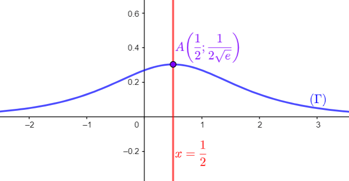
- Représenter graphiquement la courbe $(\Gamma)$.
(On prendra $\left\|\vec{i}\right\|=1\,cm,\, \left\|\vec{j}\right\|=2\,cm,\,\dfrac{1}{2\sqrt{e}} \approx 0.30, \dfrac{1}{1+e} \approx 0.27$).
-
- Montrer que : $\displaystyle\int_{0}^{1/2} f(x)\, dx = \int_{1/2}^1 f(x)\, dx$.
- En déduire que $\displaystyle\int_{0}^{1} f(x)\, dx = 2 \int_{0}^{1/2} f(x)\, dx$.
-
- En effectuant le changement de variable : $t = e^x $, montrer que : $$\int_{0}^{1/2} f(x)\, dx = \int_{1}^{\sqrt{e}} \dfrac{dt}{t^2 + e}.$$
- Montrer que : $$\int_{0}^{1/2} f(x)\, dx = \dfrac{1}{\sqrt{e}} \left(\arctan\left(\sqrt{e}\right)-\dfrac{\pi}{4}\right).$$
- En déduire l’aire, en $cm^2$, du domaine plan délimité par $(\Gamma)$, les droites d’équations respectives : $ x=0$, $x=1$, et $y=0$.
Partie II :
On considère la suite $(u_n)_{n\in\mathbb{N}}$ définie par :
$$u_0 \in \left]0; \dfrac{1}{2}\right[,\, \text{ et }\, \left(\forall n \in \mathbb{N}\right);\,\, u_{n+1} = f(u_n)$$
- En utilisant le résultat de la question I.2-a), montrer que :
$$\left(\forall x \in \mathbb{R}\right);\,\, |f'(x)| \leq f(x)$$
-
- Montrer que :
$$\left(\forall x \in \left[0; \dfrac{1}{2}\right]\right);\,\, 0 \leq f'(x) < \dfrac{1}{2}$$
- Montrer que la fonction $g : x\mapsto g(x)=f(x)-x$ est strictement décroissante sur $\mathbb{R}$.
- En déduire qu’il existe un unique réel $\alpha \in \left]0;\dfrac{1}{2}\right[$ tel que : $f(\alpha)=\alpha$
-
- Montrer que : $\left(\forall n \in \mathbb{N}\right); \quad 0 < u_n < \dfrac{1}{2}$
- Montrer que : $\left(\forall n \in \mathbb{N}\right); \quad |u_{n+1}-\alpha| \leq \dfrac{1}{2} |u_n-\alpha|$
- Montrer par récurrence que : $\left(\forall n \in \mathbb{N}\right); \quad |u_n-\alpha| \leq \left( \dfrac{1}{2} \right)^{n+1}$
- En déduire que la suite $(u_n)_{n \in \mathbb{N}}$ converge vers $\alpha$
Partie III :
On considère la suite numérique $(S_n)_{n \in \mathbb{N}}$ définie par : \[\left( {\forall n \in {\mathbb{N}^*}} \right);\quad {S_n} = \frac{1}{{n\left( {n + 1} \right)}}\sum\limits_{k = 1}^{k = n} {\frac{k}{{{e^{\frac{k}{n}}} + {e^{\frac{{n-k}}{n}}}}}} \]
-
- Vérifier que : $\left( {\forall n \in {\mathbb{N}^*}} \right);\quad {S_n} = \dfrac{1}{{n + 1}}\displaystyle\sum\limits_{k = 1}^{k = n} {\dfrac{k}{n}f\left( {\dfrac{k}{n}} \right)} $
- Montrer que: $$\displaystyle\int_0^1 x f(x) \, dx = \int_0^{1/2}f(x) \, dx$$
(On pourra effectuer le changement de variable : $t = 1-x$)
- Montrer que la suite $(S_n)_{n \in \mathbb{N}}$ est convergente et déterminer sa limite.
Indication
Partie I :
-
- Évident.
- Utiliser la définition de $f$ pour montrer la symétrie de $f$ autour de $x = \dfrac{1}{2}$.
- Montrer que : $\mathop {\lim }\limits_{x \to -\infty } f\left( x \right) = 0$, puis poser : $x=1-y$, pour calculer : $\mathop {\lim }\limits_{x \to + \infty } f\left( x \right)$.
- Interpréter graphiquement ces limites comme des asymptotes horizontales.
-
- Calculer la dérivée $f'(x)$ en utilisant la règle du quotient et simplifier l’expression.
- Remarquer que le singne de $f'(x)$ est celui de $1-e^{2x-1}$, puis en déduire que $f$ admet une valeur maximale.
- Tracer la courbe en utilisant les informations précédentes et les valeurs approchées données.
-
- Faire un changement de variable, puis utiliser la propriété de symétrie trouvée en I.1-a).
- Utiliser la somme des deux intégrales pour exprimer $\displaystyle\int_0^1 f(x) dx$.
-
- Effectuer un changement de variable en posant: $t=e^x$.
- Utiliser une primitive liée à l’arctangente pour calculer explicitement l’intégrale.
- Remarque que : $\mathcal{A} = \displaystyle\int\limits_0^1 {\left|
{f\left( x \right)} \right|dx \times \left\| {\overrightarrow i }
\right\| \times \left\| {\overrightarrow j } \right\|}$.
Partie II :
- Utiliser la formule de $f'(x)$ pour estimer la valeur absolue de la dérivée en fonction de $f(x)$, puis remarque que : $\left| {1 -{e^{2x -1}}} \right| \le \left| {1 + {e^{2x -1}}} \right|$.
-
- Utiliser les questions I-2)b) et II-1).
- Étudier le signe de la dérivée de $g(x) = f(x) -x$ pour conclure sur sa décroissance.
- Montrer que $g$ est une bijection de $\mathbb{R}$ vers $\mathbb{R}$, puis conclure.
-
- Montrer par récurrence que la suite $(u_n)$ reste dans l’intervalle $\left]0, \dfrac{1}{2}\right[$.
- Appliquer le théorème des accroissements finis à la fonction $f$.
- Prouver par récurrence la majoration explicite de cette distance.
- Conclure la convergence de la suite.
Partie III :
-
- Remarquer que : $f\left( {\frac{k}{n}} \right) = \dfrac{1}{{{e^{\frac{k}{n}}} + {e^{\frac{{n -k}}{n}}}}}$.
- Utiliser un changement de variable $t=1-x$ pour montrer l’égalité.
- Utiliser la propriété des sommes de Riemann pour montrer la convergence de $(S_n)$ et calculer la limite comme une intégrale connue.
Corrigé
Partie I :
-
-
Pour tout $x \in \mathbb{R},$ on a:
$$\begin{aligned} f\left( {1-x}\right)&= \frac{{{e^{1 -x}}}}{{{e^{2 -2x}} + e}}= \frac{{e\times {e^{ -x}}}}{{{e^2}{e^{ -2x}} + e}}\\
&= \frac{{{e^{-x}}}}{{e{e^{ -2x}} + 1}}= \frac{1}{{e{e^{ -x}} + {e^x}}}\\
&=\frac{1}{{{e^{ -x}}\left( {e + {e^{2x}}} \right)}}= \frac{1}{{{e^{-x}}\left( {e + {e^{2x}}} \right)}} \\
&= f\left( x \right)
\end{aligned}$$ D’où : $$\boxed{\left(\forall x \in \mathbb{R}\right);~~f\left( {1-x}\right)=f(x)}$$
-
Pour tout $x \in \mathbb{R},$ on a : $1-x \in \mathbb{R}$ et
$f(1-x)=f(x)$, cela signifie que :
$$\boxed{\text{ la courbe } (\Gamma) \text{ de la fonction }
f \text{ est symétrique par rapport à la droite }
x=\dfrac{1}{2}.}$$
-
Calculons $\displaystyle\lim_{x \to-\infty} f(x)$ puis
$\displaystyle\lim_{x \to+\infty} f(x)$. On a : $$\mathop {\lim
}\limits_{x \to -\infty } {e^{2x}} = \mathop {\lim }\limits_{x \to
-\infty } {e^x} = 0$$ Alors : $$\mathop {\lim }\limits_{x \to
-\infty } f\left( x \right) = \mathop {\lim }\limits_{x \to -\infty
} \frac{{{e^x}}}{{{e^{2x}} + e}} = \frac{0}{{0 + e}} = 0$$ On pose :
$x=1-y$, alors : $\left( {x \to + \infty } \right) \Leftrightarrow
\left( {y \to -\infty } \right)$, alors, on a : $$\mathop {\lim
}\limits_{x \to + \infty } f\left( x \right) = \mathop {\lim
}\limits_{y \to -\infty } f\left( {1 -y} \right) = \mathop {\lim
}\limits_{y \to -\infty } f\left( y \right) = 0$$ Finalement : $$\boxed{\displaystyle\lim_{x \to-\infty} f(x) =\displaystyle\lim_{x \to +\infty} f(x)=0}$$
-
Comme $\mathop {\lim }\limits_{x \to + \infty } f\left( x \right) =
\mathop {\lim }\limits_{x \to -\infty } f\left( x \right) = 0$,
alors l’axe des abscisses est une asymptote horizontale à la courbe
$(\Gamma)$ au voisinage de $-\infty$ et au voisinage de $+\infty$.
-
-
La fonction $f$ est la composition et le quotient de fonctions
dérivables sur $\mathbb{R}$, avec un dénominateur qui ne s’annule
jamais, donc, $f$ est dérivable sur $\mathbb{R}$, alors pour tout
$x\in\mathbb{R}$, on a : \[\begin{aligned} f'(x) &=
\frac{{{e^x}\left( {{e^{2x}} + e} \right) -{e^x}\left( {2{e^{2x}}}
\right)}}{{{{\left( {{e^{2x}} + e} \right)}^2}}} =
\frac{{{e^x}\left( {{e^{2x}} + e -2{e^{2x}}} \right)}}{{\left(
{{e^{2x}} + e} \right)\left( {{e^{2x}} + e} \right)}}\\ &=
f\left( x \right)\frac{{e -{e^{2x}}}}{{e + {e^{2x}}}} = f\left( x
\right)\frac{{e\left( {1 -{e^{2x -1}}} \right)}}{{e\left( {1 +
{e^{2x -1}}} \right)}}\\ &= f\left( x \right)\frac{{1 -{e^{2x
-1}}}}{{1 + {e^{2x -1}}}} \end{aligned}\] Finalement : $$\boxed{(\forall x\in\mathbb{R});~~f'(x)=f\left( x \right)\frac{{1 -{e^{2x
-1}}}}{{1 + {e^{2x -1}}}}}$$
-
Soit $x\in\mathbb{R}$, on a : $$e^x>0, ~\text{ et }~ e^{2x}+e>0,$$
donc $\dfrac{{{e^x}}}{{{e^{2x}} + e}}>0$, donc $f(x)>0$, et comme : $1+e^{2x-1}>0,$
donc le signe de $f'(x)$ est celui de $1-e^{2x-1}$.
On a : \[\begin{aligned} 1 -{e^{2x -1}} > 0
&\Leftrightarrow {e^{2x -1}} < 1\\ &\Leftrightarrow 2x -1
< 0\\ &\Leftrightarrow 2x < 1\\ &\Leftrightarrow x
< \frac{1}{2} \end{aligned}\]
Si $x \le \dfrac{1}{2}$, alors : $f'(x)\ge 0$, alors $f$ est croissante sur $\left]-\infty;\dfrac{1}{2}\right]$.
Si $x \ge \dfrac{1}{2}$, alors :
$f'(x)\le 0$, alors $f$ est décroissante sur $\left[\dfrac{1}{2};+\infty\right[$.
Finalement :
$$\boxed{f \text{ est croissante sur } \left]-\infty;\dfrac{1}{2}\right[ \text{ et décroissante sur } \left[\dfrac{1}{2};+\infty\right[}$$ Par suite, la fonction $f$ admet une valeur maximale en $\dfrac{1}{2}$ sur $\mathbb{R}$, donc, pour
tout $x\in\mathbb{R}$, $$f(x)\le f\left(\dfrac{1}{2}\right)$$ et on a :
\[f\left( {\frac{1}{2}} \right) = \frac{{{e^{1/2}}}}{{e + e}} =
\frac{{{e^{1/2}}}}{{2e}} = \frac{1}{{2\sqrt e }} < \frac{1}{2}\] Donc : $$\boxed{\left(\forall x \in \mathbb{R}\right);~~0 < f(x) <
\dfrac{1}{2}.}$$
-
La courbe $(\Gamma)$ de la fonction $f$.
-
-
Posons $u=1−x$, alors : $dx=-du$,
$$\left\{ \begin{aligned}
&\left( {x \to 0} \right) \Leftrightarrow \left( {u \to 1} \right)\\
&\left( {x \to \frac{1}{2}} \right) \Leftrightarrow \left( {u \to \frac{1}{2}} \right)
\end{aligned} \right.$$ Alors : $$\begin{aligned}
\int\limits_0^{1/2} {f\left( x \right)dx} &=
\int\limits_1^{1/2} { -f\left( {1 -u} \right)du}\\
&=\int\limits_{1/2}^1 {f\left( {1 -u} \right)du}\\
&= \int\limits_{1/2}^1{f\left( u \right)du}
\end{aligned}$$ Car $f(1-u)=f(u)$, alors :
$$\boxed{\displaystyle\int_{0}^{1/2} f(x)\, dx = \int_{1/2}^1 f(x)\, dx}$$
- On a :
\[\begin{aligned} \int\limits_0^1 {f\left( x \right)dx} &=
\int\limits_0^{1/2} {f\left( x \right)dx} + \int\limits_{1/2}^1
{f\left( x \right)dx} \\ &= \int\limits_0^{1/2} {f\left( x
\right)dx} + \int\limits_0^{1/2} {f\left( x \right)dx} \\ &=
2\int\limits_0^{1/2} {f\left( x \right)dx} \end{aligned}\] Donc : $$\boxed{\int\limits_0^1 {f\left( x \right)dx} =2\int\limits_0^{1/2} {f\left( x \right)dx}}$$
-
-
On pose : $t = e^x $, alors : \[t = {e^x} \Leftrightarrow \ln t = x
\Rightarrow \frac{dt}{t} = dx\]
Alors : \[\left\{ \begin{aligned}
&\left( {x \to 0} \right) \Leftrightarrow \left( {t \to 1} \right)\\
&\left( {x \to \frac{1}{2}} \right) \Leftrightarrow \left( {t \to \sqrt e } \right)
\end{aligned} \right.\] Donc : \[\begin{aligned} \int\limits_0^{1/2} {f\left( x
\right)dx} &= \int\limits_1^{\sqrt e } {\frac{{f\left( {\ln t}
\right)}}{t}dt} \\ &= \int\limits_1^{\sqrt e }
{\frac{1}{t}\left( {\frac{{{e^{\ln t}}}}{{{e^{2\ln t}} + e}}}
\right)dt} \\ &= \int\limits_1^{\sqrt e } {\frac{1}{t}\left(
{\frac{t}{{{t^2} + e}}} \right)dt} \\ &= \int\limits_1^{\sqrt e
} {\frac{{dt}}{{{t^2} + e}}} \end{aligned}\] Donc:
$$\boxed{\int_{0}^{1/2} f(x)\, dx = \int_{1}^{\sqrt{e}} \dfrac{dt}{t^2 +
e}.}$$
-
On a : $$\begin{aligned} \int\limits_0^{1/2} {f\left( x \right)}
&= \int\limits_1^{\sqrt e } {\frac{{dt}}{{{t^2} + e}}} \\
&=\frac{1}{{\sqrt e }}\int\limits_1^{\sqrt e } {\frac{{\frac{1}{{\sqrt
e }}}}{{e\left( {1 + {{\left( {\frac{t}{{\sqrt e }}} \right)}^2}}
\right)}}dt} \\
&= \frac{1}{{\sqrt e }}\Big[ {\arctan t}
\Big]_1^{\sqrt e }\\
&= \frac{1}{{\sqrt e }}\left( {\arctan
\sqrt e -\arctan 1} \right)\\
&= \frac{1}{{\sqrt e }}\left(
{\arctan \sqrt e -\frac{\pi }{4}} \right) \end{aligned}$$ Donc :
$$\boxed{\int_{0}^{1/2} f(x)\, dx = \dfrac{1}{\sqrt{e}}
\left(\arctan\left(\sqrt{e}\right)-\dfrac{\pi}{4}\right).}$$
- L’aire $\mathcal{A}$ du domaine plan délimité par $(\Gamma)$, les droites $x=0$, $x=1$ et $y=0$ est:
\[\begin{aligned} \mathcal{A} &= \int\limits_0^1 {\left|
{f\left( x \right)} \right|dx \times \left\| {\overrightarrow i }
\right\| \times \left\| {\overrightarrow j } \right\|} \\ &=
\int\limits_0^1 {f\left( x \right)dx \times 1cm \times 2cm}
\quad\Big(\text{ car }\,\,f\left( x \right) > 0\Big)\\ &=
2\int\limits_0^{1/2} {f\left( x \right)dx \times 2c{m^2}} \\ &=
4\int\limits_0^{1/2} {f\left( x \right)dx \times c{m^2}} \\ &=
\frac{4}{{\sqrt e }}\left( {\arctan \sqrt e -\frac{\pi }{4}}
\right)c{m^2} \end{aligned}\] Donc : $$\boxed{\mathcal{A}=\frac{4}{{\sqrt e }}\left( {\arctan \sqrt e -\frac{\pi }{4}}
\right)c{m^2}}$$
Partie II :
On considère la suite $(u_n)_{n\in\mathbb{N}}$ définie par : $$u_0 \in
\left]0; \dfrac{1}{2}\right[,\, \text{ et }\, \left(\forall n \in
\mathbb{N}\right);\,\, u_{n+1} = f(u_n)$$
-
D’après le résultat de la question $I)2)a)$, on a, pour tout $x \in \mathbb{R}$:
$$\left| {f’\left( x \right)} \right| = f\left( x \right)\left|
{\frac{{1 -{e^{2x -1}}}}{{1 + {e^{2x -1}}}}} \right|\quad\Big(\text{ car }\,\,f\left( x \right) > 0\Big)$$ On a :
$$\begin{aligned}
\left| {1 -{e^{2x -1}}} \right| \le \left| {1 + {e^{2x -1}}} \right|
&\Leftrightarrow \left| {\frac{{1 -{e^{2x -1}}}}{{1 + {e^{2x -1}}}}}
\right| \le 1\\ &\Leftrightarrow f\left( x \right)\left| {\frac{{1
-{e^{2x -1}}}}{{1 + {e^{2x -1}}}}} \right| \le f\left( x \right)\\
&\Leftrightarrow \left| {f’\left( x \right)} \right| \le f\left( x
\right) \end{aligned}$$ Donc : $$\boxed{\left(\forall x \in \mathbb{R}\right);\quad\left| {f’\left( x \right)} \right| \le f\left( x
\right)}$$
-
-
D’après la question $I)2)b)$, pour $x\le \dfrac{1}{2}$, on a : $f'(x)\ge
0$, et d’après les questions $I)2)b)$ et $II)1)$, pour tout $x\in\mathbb{R}$, ona : $f'(x)\le f(x)<
\dfrac{1}{2}$, alors: $$\boxed{\left(\forall x \in \left[0;
\dfrac{1}{2}\right]\right);\quad 0 \leq f'(x) < \dfrac{1}{2}}$$
-
La fonction $g(x)=f(x)−x$ est dérivable sur $\mathbb{R}$ comme
différence de deux fonctions dérivables sur $\mathbb{R}$. On a :
$$g’\left( x \right) = f’\left( x \right) -1,$$ Pour tout $x\in\mathbb{R}$, on a:
\[\begin{aligned}
\left| {f’\left( x \right)} \right| \le f\left( x \right) < \frac{1}{2} &\Rightarrow f'\left( x \right) < \frac{1}{2}\\
&\Rightarrow f'\left( x \right) -1 < \frac{1}{2} -1\\
&\Rightarrow f'\left( x \right) -1 < -\frac{1}{2}\\
&\Rightarrow g'\left( x \right) < 0
\end{aligned}\]
Donc : $$\boxed{g : x\mapsto g(x)=f(x)-x \text{ est strictement décroissante sur }\mathbb{R}}$$
-
La fonction $g$ est continue et strictement décroissante sur $\mathbb{R}$,
donc $g$ est une bijection de $\mathbb{R}$ vers $J$ tel que:\[J =
\left] {\mathop {\lim }\limits_{x \to + \infty } g\left( x
\right);\mathop {\lim }\limits_{x \to -\infty } g\left( x \right)}
\right[ = \left] { -\infty ; + \infty } \right[\] et comme $0\in
g\left( {\left] { -\infty ; + \infty } \right[} \right)$, alors :
\[\left( {\exists !\alpha \in \mathbb{R}} \right);\,\,\,g\left(
\alpha \right) = 0\] C’est-à-dire : \[\left( {\exists !\alpha \in
\mathbb{R}} \right);\,\,\,f\left( \alpha \right) = \alpha\] et puisque : $$\begin{aligned} &g\left( 0 \right) = f\left( 0
\right) -0 = \frac{1}{{1 + e}} > 0\\ &g\left( {\frac{1}{2}}
\right) = f\left( {\frac{1}{2}} \right) -\frac{1}{2} =
\frac{1}{{2\sqrt e }} -\frac{1}{2} = \frac{1}{2}\left(
{\frac{1}{{\sqrt e }} -1} \right) < 0 \end{aligned}$$ donc
\[g\left( 0 \right) \times g\left( {\frac{1}{2}} \right) < 0\] Alors : $$\boxed{\left(\exists!\alpha \in
\left]0;\dfrac{1}{2}\right[\right);\quad f(\alpha)=\alpha}$$
-
-
Pour $n=0$, on a : $0 < u_0 <
\dfrac{1}{2}$
Soit $n\in\mathbb{N}$, on suppose que : $0 < u_n<
\dfrac{1}{2}$ et montrons que : $0 < u_{n+1}<
\dfrac{1}{2}$D’après I)2)b), pour tout $x\in\mathbb{R}$, $0 <
f(x) < \dfrac{1}{2}$, et comme ${u_n} \in \left] {0;\dfrac{1}{2}}
\right[ \subset \mathbb{R}$, alors : $0 < f(u_n) <
\dfrac{1}{2}$, alors : $0 < u_{n+1} < \dfrac{1}{2}$
Alors :
$$\boxed{\left(\forall n \in \mathbb{N}\right); \quad 0 < u_n <
\dfrac{1}{2}}$$
-
Soit $n\in\mathbb{N}$, on a $f$ est continue sur l’intervalle fermé
d’extrémités $u_n$ et $\alpha$. La fonction $f$ est dérivable sur
l’intervalle ouvert d’extrémités $u_n$ et $\alpha$. Donc d’après le
T.A.F, on déduit que : \[\left( {\exists c \in \left] {\min \left(
{{u_n},\alpha } \right);\max \left( {{u_n},\alpha } \right)}
\right[} \right);\,\,\,\,f\left( {{u_n}} \right) -f\left( \alpha
\right) = f’\left( c \right)\left( {{u_n} -\alpha } \right)\] alors : \[\left| {f\left( {{u_n}} \right) -f\left( \alpha \right)}
\right| = \left| {f’\left( c \right)} \right|\left| {{u_n} -\alpha
} \right|\] Or : \[\left( {\forall x \in \left[ {0;\frac{1}{2}}
\right]} \right);\,\,\,\,\left| {f’\left( x \right)} \right| \le
\frac{1}{2}\] alors : \[\left| {f’\left( c \right)} \right| \le
\frac{1}{2}\] alors : \[\left| {f\left( {{u_n}} \right) -f\left(
\alpha \right)} \right| \le \frac{1}{2}\left| {{u_n} -\alpha }
\right|\] alors : \[\left| {{u_{n + 1}} -\alpha } \right| \le
\frac{1}{2}\left| {{u_n} -\alpha } \right|\] D’où :
$$\boxed{\left(\forall n \in \mathbb{N}\right); \quad
|u_{n+1}-\alpha| \leq \dfrac{1}{2} |u_n-\alpha|}$$
-
Pour
$n=0$, on a :
\[\begin{aligned}
\left\{ \begin{array}{l}
0 < {u_0} < \dfrac{1}{2}\\
0 < \alpha < \dfrac{1}{2}
\end{array} \right. &\Rightarrow 0 -\frac{1}{2} < {u_0} -\alpha < \frac{1}{2} -0\\
&\Rightarrow -\frac{1}{2} < {u_0} -\alpha < \frac{1}{2}\\
&\Rightarrow \left| {{u_0} -\alpha } \right| < \frac{1}{2}
\end{aligned}\]
Soit $n\in\mathbb{N}$. On suppose
que \[\left| {{u_n} -\alpha } \right| < {\left( {\frac{1}{2}}
\right)^{n + 1}}\] et on montre que : \[\left| {{u_{n+1}} -\alpha }
\right| < {\left( {\frac{1}{2}} \right)^{n + 2}}\] On a : \[\left|
{{u_n} -\alpha } \right| < {\left( {\frac{1}{2}} \right)^{n +
1}},\] alors : \[\frac{1}{2}\left| {{u_n} -\alpha } \right| <
{\left( {\frac{1}{2}} \right)^{n + 2}}\] et comme : \[\left| {{u_{n
+ 1}} -\alpha } \right| < \frac{1}{2}\left| {{u_n} -\alpha }
\right|\] donc : \[\left| {{u_{n + 1}} -\alpha } \right| < {\left(
{\frac{1}{2}} \right)^{n + 2}}\] Donc, d'après le principe de
récurrence : \[\boxed{\left( {\forall n \in \mathbb{N}}
\right);\,\,\,\,\,\,\left| {{u_n} -\alpha } \right| < {\left(
{\frac{1}{2}} \right)^{n + 1}}}\]
- On a :
\[\lim {\left( {\frac{1}{2}} \right)^{n + 1}} = 0\,\,\,\,\,\left( {car\,\, -1 < \frac{1}{2} < 1} \right)\]
Alors : \[\lim \left| {{u_n} -\alpha } \right| = 0\,\,\,\,\left( {car\,\,\left| {{u_n} -\alpha } \right| < {{\left( {\frac{1}{2}} \right)}^{n + 1}}} \right)\]
Donc : \[\lim {u_n} = \alpha\]
D'où : $$\boxed{\text{la suite } (u_n)_{n \in \mathbb{N}} \text{ converge vers }
\alpha}$$
Partie III :
On considère la suite numérique $(S_n)_{n \in \mathbb{N}}$ définie par :
\[\left( {\forall n \in {\mathbb{N}^*}} \right);\quad {S_n} =
\frac{1}{{n\left( {n + 1} \right)}}\sum\limits_{k = 1}^{k = n}
{\frac{k}{{{e^{\frac{k}{n}}} + {e^{\frac{{n-k}}{n}}}}}} \]
-
-
Soit
$n\in\mathbb{N}^*$, on a : $$\begin{aligned} {S_n} &=
\frac{1}{{n\left( {n + 1} \right)}}\sum\limits_{k = 1}^{k = n}
{\frac{k}{{{e^{\frac{k}{n}}} + {e^{\frac{{n -k}}{n}}}}}} \\ &=
\frac{1}{{n + 1}}\sum\limits_{k = 1}^{k = n} {\frac{k}{n} \times
\frac{1}{{{e^{\frac{k}{n}}} + {e^{\frac{{n -k}}{n}}}}}} =
\frac{1}{{n + 1}}\sum\limits_{k = 1}^{k = n} {\frac{k}{n} \times
\frac{1}{{{e^{\frac{k}{n}}} + {e^{1 -\frac{k}{n}}}}}} \\ &=
\frac{1}{{n + 1}}\sum\limits_{k = 1}^{k = n} {\frac{k}{n} \times
\frac{1}{{{e^{ -\frac{k}{n}}}\left( {{e^{\frac{{2k}}{n}}} + e}
\right)}} = } \frac{1}{{n + 1}}\sum\limits_{k= 1}^{k = n}
{\frac{k}{n} \times \frac{{{e^{\frac{k}{n}}}}}{{{e^{\frac{{2k}}{n}}}
+ e}}} \\ &= \frac{1}{{n + 1}}\sum\limits_{k = 1}^{k = n}
{\frac{k}{n} \times f\left( {\frac{k}{n}} \right)} \end{aligned}$$ Donc :
$$\boxed{\left(\forall n\in\mathbb{N}^*\right);\quad {S_n}=\frac{1}{{n + 1}}\sum\limits_{k = 1}^{k = n}
{\frac{k}{n} \times f\left( {\frac{k}{n}} \right)}}$$
-
On pose : \[I = \int_0^1 {xf\left( x \right)dx} \]
On pose $t=1-x$, alors $dt=-dx$, et on a :
\[\left\{ \begin{aligned}
&x \to 0 \Leftrightarrow t \to 1\\
&x \to 1 \Leftrightarrow t \to 0
\end{aligned} \right.\] alors : \[\begin{aligned} I &= \int_1^0 {\left( {1 -t}
\right)f\left( {1 -t} \right)\left( { -dt} \right)} \\ &= \int_0^1
{\left( {1 -t} \right)f\left( {1 -t} \right)dt} \\ &= \int_0^1
{\left( {1 -t} \right)f\left( t \right)dt} \\ &= \int_0^1 {f\left(
t \right)dt} -\int_0^1 {tf\left( t \right)dt} \\ &= 2\int_0^{1/2}
{f\left( x \right)dx} -I \end{aligned}\] Alors : $$2I =
2\int_0^{1/2} {f\left( x \right)dx}$$ Alors : $$I = \int_0^{1/2}
{f\left( x \right)dx}$$ D’où :
$$\boxed{\displaystyle\int_0^1 x f(x) \, dx = \int_0^{1/2}f(x)
\, dx}$$
-
Soit $n\in\mathbb{N}^*$, on a : \[\begin{aligned}
{S_n} &= \frac{1}{{n + 1}}\sum\limits_{k = 1}^{k = n}
{\frac{k}{n}f\left( {\frac{k}{n}} \right)} \\ &= \frac{1}{{1 +
\frac{1}{n}}} \times \frac{1}{n}\sum\limits_{k = 1}^{k = n}
{\frac{k}{n}f\left( {\frac{k}{n}} \right)} \\ &= \frac{1}{{1 +
\frac{1}{n}}} \times \frac{1}{n}\sum\limits_{k = 1}^{k = n} {h\left(
{\frac{k}{n}} \right)\,\,\,\,\,\,\,\Big( {\text{ avec } h\left( x \right)
= xf\left( x \right)} \Big)} \end{aligned}\] Comme la fonction $h$ est
continue sur $[0,1]$, donc : \[\begin{aligned} \mathop {\lim }\limits_{n
\to + \infty } \frac{1}{n}\sum\limits_{k = 1}^{k = n} {h\left(
{\frac{k}{n}} \right)} &= \int_0^1 {h\left( x \right)dx} \\ &= \int_0^1
{xf\left( x \right)dx} \\ &= \int_0^{1/2} {f\left( x \right)dx} \\ &=
\frac{1}{{\sqrt e }}\left( {\arctan \sqrt e -\frac{\pi }{4}} \right)
\end{aligned}\] et comme : \[\mathop {\lim }\limits_{n \to + \infty }
\dfrac{1}{{1 + \dfrac{1}{n}}} = 1\] alors : \[\mathop {\lim }\limits_{n
\to + \infty } {S_n} = \frac{1}{{\sqrt e }}\left( {\arctan \sqrt e –
\frac{\pi }{4}} \right)\] D’où : $$\boxed{\text{la suite }(S_n)_{n\in\mathbb{N}} \text{ est convergente et tend vers }
\dfrac{1}{{\sqrt e }}\left( {\arctan \sqrt e -\dfrac{\pi }{4}}
\right)}$$
Enoncé
Soit $\alpha\in\left[0;2\pi\right[$.
On considère dans l’ensemble des nombres complexes $\mathbb{C}$ l’équation $(E_\alpha)$ d’inconnue $z$ : $$(E_\alpha) : \quad z^2-2^\alpha e^{i\alpha}(1 + 2i)z + i2^{2\alpha + 1} e^{i2\alpha} = 0$$
Partie I:
-
- Vérifier que le discriminant de l’équation $(E_\alpha)$ est : $$\Delta_\alpha = \left(2^{\alpha}e^{i\alpha}(1-2i)\right)^2$$
- En déduire les deux solutions $a$ et $b$ de l’équation $(E_\alpha)$ avec $|a| < |b|$
- Vérifier que $\dfrac{b}{a}$ est un imaginaire pur.
Partie II:
Le plan complexe est rapporté à un repère orthonormé direct $(O ; \vec{u}, \vec{v})$.
On note par $M(z)$ le point d’affixe le nombre complexe $z$.
On pose $\dfrac{b}{a}=\lambda i$ avec $\lambda=\operatorname{Im}\left(\dfrac{b}{a}\right)$.
- On considère les points $A(a), B(b)$ et $H(h)$ avec $\dfrac{1}{h}=\dfrac{1}{a}+\dfrac{1}{b}$.
- Montrer que $: \dfrac{h}{b-a}=-\left(\dfrac{\lambda}{\lambda^2+1}\right) i$ puis en déduire que les droites $(O H) \operatorname{et}(A B)$ sont perpendiculaires.
- Montrer que : $\dfrac{h-a}{b-a}=\dfrac{1}{\lambda^2+1}$ puis en déduire que les points $H, A$ et $B$ sont alignés.
- Soient $I(m)$ le milieu du segment $[O H]$ et $J(n)$ le milieu du segment $[H B]$.
- Montrer que : $\dfrac{n}{m-a}=-\lambda i$.
- En déduire que les droites $(O J)$ et $(A I)$ sont perpendiculaires et que $O J=|\lambda| A I$.
- Soit $K$ le point d’intersection des droites ( $O J$ ) et ( $A I$ )Montrer que les points $K, I, H$ et $J$ sont cocycliques.
- Montrer que les droites $(I J)$ et $(O A)$ sont perpendiculaires.
Indication
Partie I – Aides :
-
-
Utiliser la formule du discriminant : $\Delta= b^2-4ac$ où $a=1$, $b=-2^\alpha e^{i\alpha}(1+2i)$ et $c=i2^{2\alpha+1}e^{i2\alpha}$. Développer en utilisant les identités algébriques et les propriétés des complexes.
-
Appliquer la formule des racines d’une équation du second degré:
$$\begin{aligned}
z_1&=\dfrac{-b+\sqrt{\Delta}}{2a}\\
z_2&=\dfrac{-b-\sqrt{\Delta}}{2a}\end{aligned}$$
Simplifier les expressions en factorisant.
-
Simplifier le quotient, et montrer que : $\dfrac{b}{a}=2i$.
Partie II – Aides :
-
-
Exprimer $b = \lambda ia$, puis utiliser la formule de $h$ en fonction de $a$ et $b$. Réécrire $\dfrac{h}{b-a}$ et simplifier. Remarquer que : $\overline {\left( {\overrightarrow {AB} ,\overrightarrow {OH} } \right)} \equiv \arg \left( {\dfrac{h}{{b -a}}} \right)\left[ {2\pi } \right]$
-
Exprimer $\dfrac{h-a}{b-a}$ et montrer que le résultat est réel.
-
-
Utiliser les formules des milieux et exprimer $m$ et $n$ en fonction de $a$ et $b$. Calculer le rapport $\dfrac{n}{m-a}$.
-
Remarquer que $\left( {OJ} \right) \bot \left( {AI} \right) \Leftrightarrow \overline {\left( {\overrightarrow {AI} ,\overrightarrow {OJ} } \right)} \equiv \pm \dfrac{\pi }{2}\left[ {2\pi } \right]$
et que : $OJ = \left| \lambda \right|AI \Leftrightarrow \left| n \right| = \left| {\lambda \left( {m -a} \right)} \right|$.
-
Comparer les rapports $\dfrac{k-m}{k-n}$ et $\dfrac{h-n}{h-m}$. Vérifier qu’ils sont tous deux imaginaires purs.
-
Exprimer le rapport $\dfrac{z_A-z_O}{z_J-z_I}$ en fonction de $a$ et $b$, et montrer qu’il est imaginaire pur pour conclure à une orthogonalité.
Corrigé
Partie I :
-
-
Calculons le discriminant de l’équation quadratique : \[
\Delta_\alpha = \left( 2^\alpha e^{i\alpha} (1 + 2i) \right)^2 -4
\times 1 \times i 2^{2\alpha + 1} e^{i 2 \alpha}. \] Développons :
$$\begin{aligned} \Delta &= {b^2} -4ac = {\left[ {{2^\alpha
}{e^{i\alpha }}\left( {1 + 2i} \right)} \right]^2} -4i{2^{2\alpha +
1}}{e^{i2\alpha }}\\ &= {2^{2\alpha }}{e^{2i\alpha }}\left( {4i
-3} \right) -4i{2.2^{2\alpha }}.{e^{i2\alpha }}\\ &= {2^{2\alpha
}}{e^{2i\alpha }}\left( {4i -3 -8i} \right)\\ &= {2^{2\alpha
}}{e^{2i\alpha }}\left( { -3 -8i} \right)\\ &= {\left[
{{2^\alpha }{e^{i\alpha }}\left( {1 -2i} \right)} \right]^2}
\end{aligned}$$ Ainsi, on a bien : $$\boxed{\Delta_\alpha = \left(
2^\alpha e^{i\alpha} (1 -2i) \right)^2}.$$
-
Détermination des solutions $a$ et $b$. Les solutions de
$(E_\alpha)$ sont données par : $$z = \frac{2^\alpha e^{i\alpha} (1
+ 2i) \pm 2^\alpha e^{i\alpha} (1 -2i)}{2}.$$ Calculons chaque solution : $$\begin{cases} a = z_1 = \dfrac{2^\alpha e^{i\alpha} (1
+ 2i + 1 -2i)}{2} = 2^\alpha e^{i\alpha}, \\ b = z_2 =
\dfrac{2^\alpha e^{i\alpha} (1 + 2i -(1 -2i))}{2} = 2^{\alpha + 1}
i e^{i\alpha}. \end{cases}$$ On a $|a| = 2^\alpha$ et $|b| =
2^{\alpha + 1}$, donc $|a| < |b|$.
-
Vérification que $\dfrac{b}{a}$ est imaginaire pur : $$\frac{b}{a} =
\frac{{{2^{\alpha + 1}}i{e^{i\alpha }}}}{{{2^\alpha }{e^{i\alpha }}}} =
2i,$$ qui est bien un imaginaire pur.
Partie II :
-
-
On a : \[\frac{b}{a} = \lambda i \Leftrightarrow b = \lambda ia\] Et
on a : \[\frac{1}{h} = \frac{1}{a} + \frac{1}{b} \Leftrightarrow
\frac{1}{h} = \frac{{a + b}}{{ab}} \Leftrightarrow h =
\frac{{ab}}{{a + b}}\] Alors : \[\frac{h}{{b -a}} =
\frac{{ab}}{{\left( {a + b} \right)\left( {b -a} \right)}} =
\frac{{\lambda i{a^2}}}{{{b^2} -{a^2}}} = \frac{{\lambda i{a^2}}}{{
-{\lambda ^2}{a^2} -{a^2}}} = \frac{{\lambda i{a^2}}}{{ -{a^2}\left(
{\lambda + 1} \right)}} = -\left( {\frac{\lambda }{{{\lambda ^2} +
1}}} \right)i\] \[\begin{aligned} \overline {\left( {\overrightarrow
{AB} ,\overrightarrow {OH} } \right)} &\equiv \arg \left(
{\frac{{h -0}}{{b -a}}} \right)\left[ {2\pi } \right]\\ &\equiv
\arg \left( { -\frac{\lambda }{{{\lambda ^2} + 1}}i} \right)\left[
{2\pi } \right]\\ &\equiv \arg \left( { -i} \right)\left[ {2\pi
} \right]\,\,\,\,\,\left( {car\,\,\,\frac{\lambda }{{{\lambda ^2} +
1}} \in {\mathbb{R}^ + }} \right)\\ &\equiv -\frac{\pi
}{2}\left[ {2\pi } \right] \end{aligned}\] Donc : $\boxed{\left(
{OH} \right) \bot \left( {AB} \right)}$
-
On a : $b=\lambda ia$ et $\dfrac{h}{{b -a}} = -\left(
{\dfrac{\lambda }{{{\lambda ^2} + 1}}} \right)i$, alors :
\[\begin{aligned} \frac{{h -a}}{{b -a}} &= \frac{h}{{b -a}}
-\frac{a}{{b -a}}\\ &= -\left( {\frac{\lambda }{{{\lambda ^2} +
1}}} \right)i -\frac{a}{{\lambda ia -a}}\\ &= -\left(
{\frac{\lambda }{{{\lambda ^2} + 1}}} \right)i -\frac{1}{{\lambda i
-1}}\\ &= -\left( {\frac{\lambda }{{{\lambda ^2} + 1}}} \right)i
-\frac{{\left( {\lambda i + 1} \right)}}{{\left( {\lambda i -1}
\right)\left( {\lambda i + 1} \right)}}\\ &= -\left(
{\frac{\lambda }{{{\lambda ^2} + 1}}} \right)i -\frac{{\lambda i +
1}}{{ -{\lambda ^2} -1}}\\ &= -\left( {\frac{\lambda }{{{\lambda
^2} + 1}}} \right)i + \frac{{\lambda i + 1}}{{{\lambda ^2} + 1}}\\
&= \frac{{ -\lambda i + \lambda i + 1}}{{{\lambda ^2} + 1}}\\
&= \frac{1}{{{\lambda ^2} + 1}} \end{aligned}\] Puisque $\dfrac{{{z_H} -{z_A}}}{{{z_B} -{z_A}}} = \dfrac{{h -a}}{{b -a}} =\dfrac{1}{{{\lambda ^2} + 1}} \in \mathbb{R}$, donc les points $H$, $A$ et $B$ sont alignés.
-
-
On a : \[h = \frac{{ab}}{{a + b}}\]
$I(m)$ est le milieu du segment $[OH]$, alors:
\[m = \frac{h}{2} = \frac{{ab}}{{2\left( {a + b}
\right)}}\] $J(n)$ est le milieu du segment $[HB]$, alors:
\[n =
\frac{{h + b}}{2} = \frac{{2ab + {b^2}}}{{2\left( {a + b}
\right)}}\] alors, on a : \[\begin{aligned} \dfrac{n}{{m -a}} &=
\dfrac{{\dfrac{{h + b}}{2}}}{{\dfrac{h}{2} -a}}\\ &= \dfrac{{h +
b}}{{h -2a}}\\ &= \dfrac{{\dfrac{{ab}}{{a + b}} +
b}}{{\dfrac{{ab}}{{a + b}} -2a}}\\ &= \frac{{ab + ab +
{b^2}}}{{ab -2{a^2} -2ab}}\\ &= \frac{{2ab + {b^2}}}{{ -ab
-2{a^2}}}\\ &= -\frac{b}{a} \times \frac{{\left( {2a + b}
\right)}}{{\left( {b + 2a} \right)}}\\ &= -\frac{b}{a}\\ &=
-\lambda i \end{aligned}\] D’où : $$\boxed{\dfrac{n}{m-a}=-\lambda i}$$
-
On a : \[\begin{aligned} \overline {\left( {\overrightarrow {AI}
,\overrightarrow {OJ} } \right)} &\equiv \arg \left( {\frac{{n
-0}}{{m -a}}} \right)\left[ {2\pi } \right]\\ &\equiv \arg
\left( {\frac{n}{{m -a}}} \right)\left[ {2\pi } \right]\\
&\equiv \arg \left( { -\lambda i} \right)\left[ {2\pi }
\right]\\ &\equiv -\frac{\pi }{2}\left[ {2\pi } \right]
\end{aligned}\] Donc : \[\boxed{\left( {OJ} \right) \bot \left( {AI}
\right)}\] et on a : \[\begin{aligned} \frac{n}{{m -a}} = -\lambda i
&\Rightarrow \left| {\frac{n}{{m -a}}} \right| = \left| {
-\lambda i} \right|\\ &\Rightarrow \left| {\frac{n}{{m -a}}}
\right| = \left| \lambda \right|\\ &\Rightarrow \left| {\frac{{n
-0}}{{m -a}}} \right| = \left| \lambda \right|\\ &\Rightarrow
\left| {n -0} \right| = \left| \lambda \right|\left| {m -a}
\right|\\ &\Rightarrow OJ = \left| \lambda \right|AI
\end{aligned}\] Donc : $$\boxed{OJ = \left| \lambda \right|AI}$$
-
D’une parte, on a : $(OJ)\perp (AI)$ et comme $k \in \left( {OJ}
\right) \cap \left( {AI} \right)$, donc : $(KJ)\perp (KI),$ donc :
$$\boxed{\dfrac{k-m}{k-n}\in i\mathbb{R}}\,\,\,(*)$$ D’autre parte, on a : $(OH)\perp (AB)$ et comme les points $H$, $A$ et $B$ sont
alignés, alors : $(OH)\perp (HB)$, et puisque $I$ est le milieu de
$[OH]$ et $J$ est milieu de $[HB]$, alors : $(HI)\perp (HJ),$ donc :
$$\boxed{\dfrac{h-n}{h-m}\in i\mathbb{R}}\,\,\,(**)$$ D’après $(*)$ et $(**)$ on déduit que :
$$\dfrac{h-n}{h-m}\times\dfrac{k-m}{k-n}\in\mathbb{R}$$ Donc :
$$\boxed{\text{les points } K, I, H \text{ et } J \text{ sont cocycliques.}}$$
-
On a : \[\begin{aligned} \frac{{{z_A} -{z_O}}}{{{z_J} -{z_I}}}
&= \frac{{a -0}}{{n -m}}= \frac{a}{{\dfrac{{2ab +
{b^2}}}{{2\left( {a + b} \right)}} -\dfrac{{ab}}{{2\left( {a + b}
\right)}}}}\\ &= \frac{{2a\left( {a + b} \right)}}{{ab +
{b^2}}}= \frac{{2a\left( {a + b} \right)}}{{b\left( {a + b}
\right)}}\\ &= \frac{{2a}}{b}= \frac{2}{{\lambda i}}=
-\frac{{2i}}{\lambda } \end{aligned}\] donc : $$\dfrac{{{z_A}
-{z_O}}}{{{z_J} -{z_I}}}=-\dfrac{{2i}}{\lambda }\in i\mathbb{R},$$
donc : $$\boxed{(IJ)\perp (OA)}$$
Enoncé
Soient $p$ un nombre premier impair et $a$ un entier premier avec $p$.
- Montrer que : $\,\,a^{\frac{p-1}{2}} \equiv 1[p]$ ou $a^{\frac{p-1}{2}} \equiv-1[p]$.
- On considère dans $\mathbb{Z}$ l’équation : $\,\,a x^2 \equiv 1[p]$. Soit $x_0$ une solution de cette équation.
- Montrer que : $\,\,x_0{ }^{p-1} \equiv 1[p]$.
- En déduire que : $\,\,a^{\frac{p-1}{2}} \equiv 1[p]$.
- Soit $n$ un entier naturel non nul.
- Montrer que si $p$ divise $2^{2 n+1}-1$ alors $2^{\frac{p-1}{2}} \equiv 1[p]$.
- En déduire que l’équation $(E):\,\, 11 x+\left(2^{2 n+1}-1\right) y=1$ admet au moins une solution dans $\mathbb{Z}^2$.
- On considère dans $\mathbb{Z}$ l’équation $(F):\,\, x^2+5 x+2 \equiv 0 \quad[11]$.
- Montrer que : $\,\,(F) \Leftrightarrow 2(2 x+5)^2 \equiv 1[11]$.
- En déduire que l’équation $(F)$ n’admet pas de solution dans $\mathbb{Z}$.
Indication
-
Utilise le théorème de Fermat pour $a^{p-1} \equiv 1 \pmod{p}$, puis factorise $a^{p-1} -1$.
-
- Exprime $a x_0^2 \equiv 1 \pmod{p}$ sous forme d’une combinaison linéaire, puis applique le théorème de Bézout.
- Utilise l’égalité précédente et élève à la puissance $\dfrac{p-1}{2}$, puis applique Fermat pour $x_0^{p-1}$.
-
- Réécris la divisibilité par $p$ sous forme d’une congruence et exploite le fait que $\operatorname{pgcd}(2,p)=1$.
- Montrer que $\operatorname{pgcd}\left(11,{{2^{2n + 1}} -1} \right)=1$, puis applique le théorème de Bézout.
-
- Transforme l’équation quadratique modulo $11$ pour obtenir une forme impliquant un carré.
- Utiliser un raisonnement par l’absurde.
Corrigé
-
Puisque $p$ est premier et $p \wedge a=1$, alors, d’après le théorème de
Fermat, on a : \[{a^{p -1}} \equiv 1\left[ p \right]\] Alors :
\[\begin{aligned} {a^{p -1}} \equiv 1\left[ p \right]
&\Leftrightarrow {\left( {{a^{\frac{{p -1}}{2}}}} \right)^2} \equiv
1\left[ p \right]\\ &\Leftrightarrow p/\left( {{{\left(
{{a^{\frac{{p -1}}{2}}}} \right)}^2} -1} \right)\\ &\Leftrightarrow
p/\left( {{a^{\frac{{p -1}}{2}}} -1} \right)\left( {{a^{\frac{{p
-1}}{2}}} + 1} \right)\\ &\Leftrightarrow p/\left( {{a^{\frac{{p
-1}}{2}}} -1} \right)\,\,\text{ ou }\,\,p/\left( {{a^{\frac{{p -1}}{2}}} + 1}
\right)\,\,\,\left( {\text{ car }\,\,p\,\text{est premier }} \right)\\
&\Leftrightarrow {a^{\frac{{p -1}}{2}}} \equiv 1\left[ p
\right]\,\,\text{ ou }\,\,{a^{\frac{{p -1}}{2}}} \equiv -1\left[ p \right]
\end{aligned}\] D’où : $$\boxed{a^{\frac{{p -1}}{2}} \equiv 1\left[ p
\right]\,\,\,\text{ou}\,\,\,{a^{\frac{{p -1}}{2}}} \equiv -1\left[ p \right]}$$
-
-
On a : $a{x_0^2} \equiv 1\left[ p \right] $, alors :
$$\left( {\exists k \in \mathbb{Z}}
\right);\,\,\,\,a{x_0^2} -1 = kp, $$ alors :
$$\left( {\exists k \in
\mathbb{Z}} \right);\,\,\,\,a{x_0^2} -kp = 1, $$ alors : $$\left( {\exists
\left( {u,v} \right) \in {\mathbb{Z}^2}} \right);\,\,\,\,ux_0 + vp =
1\,\,\text{avec}\,\,u = ax_0\,\,\text{et}\,\,v = -k, $$ donc, d’après le théorème de Bezout $x_0 \wedge p = 1$ et comme $p$ est premier, donc d’après le théorème de Fermat, on a : $$\boxed{x_0^{p-1}\equiv[p]}$$
-
On a : \[a{x_0^2} \equiv 1\left[ p \right],\] alors : \[{\left(
{a{x_0^2}} \right)^{\frac{{p -1}}{2}}} \equiv 1\left[ p \right],\] alors : \[{a^{\frac{{p -1}}{2}}}{x_0^{p -1}} \equiv 1\left[ p
\right],\] comme : \[{x_0^{p-1}} \equiv 1\left[ p \right],\] alors :
\[\boxed{{a^{\frac{p-1}{2}}} \equiv 1\left[ p \right].}\]
-
-
Si $p$ divise $2^{2n+1}-1$, alors : \[\begin{aligned} p/{2^{2n + 1}}
-1 &\Leftrightarrow {2^{2n + 1}} -1 \equiv 0\left[ p \right]\\
&\Leftrightarrow {2^{2n + 1}} \equiv 1\left[ p \right]\\
&\Leftrightarrow 2 \times {\left( {{2^n}} \right)^2} \equiv
1\left[ p \right] \end{aligned}\] On a : $2 \wedge p = 1$ car $p$
est impair, et d’après la question 2) $2^n$ est solution de l’équation $2\times (2^n)^2\equiv 1[p]$, donc : $$\boxed{{2^{\frac{{p
-1}}{2}}} \equiv 1\left[ p \right]}$$
-
Puisque $11$ est premier, alors : \[11 \wedge {2^{2n + 1}} =
1\,\,\text{ ou }\,\,11 \wedge {2^{2n + 1}} -1 = 11\] Supposons que : $11
\wedge {2^{2n + 1}} -1 = 11$, alors : \[\begin{aligned} {2^{2n + 1}}
-1 \equiv 0\left[ {11} \right] &\Leftrightarrow {2^{2n + 1}}
\equiv 1\left[ {11} \right]\\ &\Leftrightarrow 2 \times {\left(
{{2^n}} \right)^2} \equiv 1\left[ {11} \right]\\
&\Leftrightarrow {2^{\frac{{11 -1}}{2}}} \equiv 1\left[ {11}
\right]\\
&\Leftrightarrow {2^5} \equiv 1\left[ {11} \right]\,\,\left(
{\text{absurde car }}{2^5} \equiv -1\left[ {11} \right] \right) \end{aligned}\] donc : $11 \wedge {2^{2n + 1}} -1
= 1$, donc d’près le théorème de Bezout, \[\boxed{\left( {\exists \left(
{x,y} \right) \in {\mathbb{Z}^2}} \right);\,\,\,\,11x + \left(
{{2^{2n + 1}} -1} \right)y = 1}\]
-
- On a :
\[\begin{aligned} {x^2} + 5x + 2 \equiv 0\left[ {11} \right]
&\Leftrightarrow 8{x^2} + 40x + 16 \equiv 0\left[ {11} \right]\\
&\Leftrightarrow 8{x^2} + 40x + 50 -50 + 16 \equiv 0\left[ {11}
\right]\\ &\Leftrightarrow 2\left( {4{x^2} + 20x + 25} \right)
-34 \equiv 0\left[ {11} \right]\\ &\Leftrightarrow 2{\left( {2x
+ 5} \right)^2} \equiv 34\left[ {11} \right]\\ &\Leftrightarrow
2{\left( {2x + 5} \right)^2} \equiv 1\left[ {11} \right]
\end{aligned}\] D’où : $$\boxed{(F)
\Leftrightarrow 2{\left( {2x + 5} \right)^2} \equiv 1\left[ {11} \right]}$$
-
Supposons que l’équation $(F)$ admette une solution dans
$\mathbb{Z}$. On a : $$(F) \Leftrightarrow 2(2x + 5)^2 \equiv 1
\left[11\right].$$ On sait que $2 \wedge 11 = 1$, donc $2x + 5$ est une solution de l’équation $2X^2 \equiv 1 \left[11\right]$, et d’après la question 2), on a : $2^{\frac{11 -1}{2}} \equiv 1
\left[11\right]$, donc : ${2^5} \equiv 1 \left[11\right]$. Or, cela
est absurde car ${2^5} = 32 \equiv -1 \left[11\right]$, donc :
$$\boxed{\text{l’équation } (F) \text{ n’admet pas de solution dans } \mathbb{Z}.}$$
Enoncé
On rappelle que $\left(M_3(\mathbb{R}),+, \times\right)$ est un anneau unitaire et non commutatif de zéro la matrice $O=\left(\begin{array}{lll}0 & 0 & 0 \\ 0 & 0 & 0 \\ 0 & 0 & 0\end{array}\right)$ et d’unité la matrice $I=\left(\begin{array}{lll}1 & 0 & 0 \\ 0 & 1 & 0 \\ 0 & 0 & 1\end{array}\right)$, et que $\left(M_3(\mathbb{R}),+,.\right)$ est un espace vectoriel réel.
Soient la matrice $A=\left(\begin{array}{ccc}-1 & -1 & 0 \\ -1 & -1 & 0 \\ -1 & 1 & -2\end{array}\right)$ et l’ensemble $E=\{M(x)=I+x A / x \in \mathbb{R}\}$
-
- Vérifier que : $\,\,A^2=-2 A$
- En déduire que : $\,\,\forall(x, y) \in \mathbb{R}^2 ;\,\, M(x) \times M(y)=M(x+y-2 x y)$
-
- Calculer : $\,\,M\left(\dfrac{1}{2}\right) \times\left(\begin{array}{lll}0 & 0 & 0 \\ 0 & 0 & 0 \\ 0 & 0 & 1\end{array}\right)$
- En déduire que la matrice $M\left(\dfrac{1}{2}\right)$ n’est pas inversible dans $\left(M_3(\mathbb{R}), \times\right)$
- Montrer que : $E-\left\{M\left(\dfrac{1}{2}\right)\right\}$ est stable pour la multiplication dans $M_3(\mathbb{R})$
(on pourra utiliser l’identité : $\left(x-\dfrac{1}{2}\right)\left(y-\dfrac{1}{2}\right)=\dfrac{-1}{2}\left(x+y-2 x y-\dfrac{1}{2}\right)$ )
- Montrer que : $\,\,\left(E-\left\{M\left(\dfrac{1}{2}\right)\right\}, \times\right)$ est un groupe commutatif.
- On munit $E$ de la loi de composition interne $T$ définie par :
$$
\forall(x, y) \in \mathbb{R}^2 ;\,\, M(x) T M(y)=M\left(x+y-\dfrac{1}{2}\right)
$$
et on considère l’application $\varphi$ définie de $\mathbb{R}$ vers $E$ par: $\forall x \in \mathbb{R} ;\,\, \varphi(x)=M\left(\dfrac{1-x}{2}\right)$
- Montrer que $\varphi$ est un homomorphisme $\operatorname{de}(\mathbb{R},+)$ vers $(E, T)$ et que $\varphi(\mathbb{R})=E$
- En déduire que ( $E, T$ ) est un groupe commutatif.
- Montrer que ( $E, T, \times$ ) est un corps commutatif.
Indication
-
-
Vérifier le calcul de $A^2$ et comparer avec $-2A$. L’objectif est de montrer la relation simple $A^2 = -2A$.
-
Développer explicitement $(I + xA)(I + yA)$ en utilisant $A^2 = -2A$ pour retrouver la forme $M(x+y-2xy)$.
-
-
Multiplier $M\left(\dfrac{1}{2}\right)$ par la matrice donnée et montrer que le produit est la matrice nulle.
-
Utiliser un raisonnement par l’absurde : si $M\left(\dfrac{1}{2}\right)$ était inversible, cela contredirait le résultat du 2)a).
-
Montrer que si $x, y \neq \dfrac{1}{2}$, alors l’expression $x+y-2xy \neq \dfrac{1}{2}$. Cela garantit la stabilité de $E \setminus \left\{M\left(\dfrac{1}{2}\right)\right\}$.
-
Vérifier les propriétés de groupe : associativité, existence de l’élément neutre $I$, commutativité, et existence d’inverses explicites $y = \dfrac{x}{2x-1}$.
-
-
Vérifier que $\varphi(x+y) = \varphi(x)~\mathrm{T}~\varphi(y)$, où $\mathrm{T}$ est la loi sur $E$.
-
Montrer la bijectivité de $\varphi$ en résolvant $\varphi(x)=M(y)$ pour $x$. En déduire que c’est un isomorphisme de groupes.
-
Conclure que $(E,\mathrm{T},\times)$ est un corps en vérifiant la distributivité de $\times$ sur $\mathrm{T}$ et les propriétés précédentes.
Corrigé
-
On a : $${A^2} = \left( {\begin{array}{*{20}{c}} { -1}&{-1}&0\\ { -1}&{ -1}&0\\ { -1}&1&{ -2}
\end{array}} \right) \times \left( {\begin{array}{*{20}{c}} {
-1}&{ -1}&0\\ { -1}&{ -1}&0\\ { -1}&1&{ -2}
\end{array}} \right) = \left( {\begin{array}{*{20}{c}}
2&2&0\\ 2&2&0\\ 2&{ -2}&4 \end{array}}
\right)$$ et \[ -2A = -2\left( {\begin{array}{*{20}{c}} { -1}&{
-1}&0\\ { -1}&{ -1}&0\\ { -1}&1&{ -2}
\end{array}} \right) = \left( {\begin{array}{*{20}{c}}
2&2&0\\ 2&2&0\\ 2&{ -2}&4 \end{array}}
\right)\] Donc : $$\boxed{A^2=-2A}$$
Pour tout $(x,y)\in\mathbb{R}^2$, on a : \[\begin{aligned} M\left( x
\right) \times M\left( y \right) &= \left( {I + xA}
\right)\left( {I + yA} \right)\\ &= {I^2} + yIA + xAI +
xy{A^2}\\ &= I + yA + xA + -2xyA\\ &= I + \left( {x + y
-2xy} \right)A\\ &= M\left( {x + y -2xy} \right) \end{aligned}\] Donc: \[\boxed{\left( {\forall \left( {x,y} \right) \in
{\mathbb{R}^2}} \right),\,\,\,\,M\left( x \right) \times M\left( y
\right) = M\left( {x + y -2xy} \right)}\]
-
On a : \[\begin{aligned} M\left( {\dfrac{1}{2}} \right) \times
\left( {\begin{array}{*{20}{c}} 0&0&0\\ 0&0&0\\
0&0&1 \end{array}} \right) &= \left( {I + \dfrac{1}{2}A}
\right)\left( {\begin{array}{*{20}{c}} 0&0&0\\
0&0&0\\ 0&0&1 \end{array}} \right)\\ &= \left(
{\begin{array}{*{20}{c}} { -\dfrac{1}{2}}&{
-\dfrac{1}{2}}&0\\ { -\dfrac{1}{2}}&{ -\dfrac{1}{2}}&0\\
{ -\dfrac{1}{2}}&{\dfrac{1}{2}}&0 \end{array}} \right)\left(
{\begin{array}{*{20}{c}} 0&0&0\\ 0&0&0\\
0&0&1 \end{array}} \right)\\ &= \left(
{\begin{array}{*{20}{c}} 0&0&0\\ 0&0&0\\
0&0&0 \end{array}} \right) \end{aligned}\] Donc :
\[\boxed{M\left( {\dfrac{1}{2}} \right) \times \left(
{\begin{array}{*{20}{c}} 0&0&0\\ 0&0&0\\
0&0&1 \end{array}} \right) = \left( {\begin{array}{*{20}{c}}
0&0&0\\ 0&0&0\\ 0&0&0 \end{array}}
\right)}\]
On suppose que $M\left( {\dfrac{1}{2}} \right)$ est inversible dans $\left( {{M_3}\left( \mathbb{R} \right), \times } \right)$, donc il existe une matrice $N$ tel que : \[M\left( {\frac{1}{2}} \right)
\times N = N \times M\left( {\frac{1}{2}} \right) = I\] et comme :
\[M\left( {\frac{1}{2}} \right) \times \left(
{\begin{array}{*{20}{c}} 0&0&0\\ 0&0&0\\
0&0&1 \end{array}} \right) = \left( {\begin{array}{*{20}{c}}
0&0&0\\ 0&0&0\\ 0&0&0 \end{array}} \right)\]
donc : \[N \times M\left( {\frac{1}{2}} \right) \times \left(
{\begin{array}{*{20}{c}} 0&0&0\\ 0&0&0\\
0&0&1 \end{array}} \right) = N \times \left(
{\begin{array}{*{20}{c}} 0&0&0\\ 0&0&0\\
0&0&0 \end{array}} \right)\] donc : \[I \times \left(
{\begin{array}{*{20}{c}} 0&0&0\\ 0&0&0\\
0&0&1 \end{array}} \right) = \left( {\begin{array}{*{20}{c}}
0&0&0\\ 0&0&0\\ 0&0&0 \end{array}} \right)\] donc : \[\left( {\begin{array}{*{20}{c}} 0&0&0\\
0&0&0\\ 0&0&1 \end{array}} \right) = \left(
{\begin{array}{*{20}{c}} 0&0&0\\ 0&0&0\\
0&0&0 \end{array}} \right)\] Ce qui est absurde, donc on déduit que : $$\boxed{M\left( {\dfrac{1}{2}} \right) \text{ n’est pas inversible dans } \left( {{M_3}\left( \mathbb{R} \right), \times
} \right)}$$
-
On a $E\backslash \left\{ {M\left( {\dfrac{1}{2}} \right)} \right\}
\subset {M_3}\left( \mathbb{R} \right)$.
Soit $M(x)$ et $M(y)$ deux éléments de $E\backslash \left\{ {M\left(
{\dfrac{1}{2}} \right)} \right\}$ tels que : $x\neq \dfrac{1}{2}$ et $x\neq \dfrac{1}{2}$
On a : $$M(x)\times M(y) = M(x+y-2xy)$$ Montrons que : $$M(x+y-2xy)\in
E\backslash \left\{ {M\left( {\dfrac{1}{2}} \right)} \right\}$$ On montre que : $$x+y-2xy\neq \dfrac{1}{2}$$ On a : $$\begin{aligned}
\left\{{\begin{array}{*{20}{c}} {x \ne \dfrac{1}{2}}\\ {y \ne
\dfrac{1}{2}} \end{array}} \right. &\Rightarrow \left\{{\begin{array}{*{20}{c}} {x -\dfrac{1}{2} \ne 0}\\ {y -\dfrac{1}{2} \ne 0} \end{array}} \right.\\ &\Rightarrow \left( {x -\dfrac{1}{2}}
\right)\left( {y -\dfrac{1}{2}} \right) \ne 0\\ &\Rightarrow
-\dfrac{1}{2}\left( {x + y -2xy -\dfrac{1}{2}} \right) \ne 0\\
&\Rightarrow x + y -2xy \ne \dfrac{1}{2} \end{aligned}$$ Donc :
$$M(x+y-2xy)\in E\backslash \left\{ {M\left( {\dfrac{1}{2}} \right)}
\right\}$$ D’où : $$\boxed{E\backslash \left\{ {M\left( {\dfrac{1}{2}}
\right)} \right\} \text{ est stable pour la multiplication dans
}{M}_3(\mathbb{R}).}$$
Montrons que : $\left( {E\backslash \left\{ {M\left( {\dfrac{1}{2}}
\right)} \right\}, \times } \right)$ est un groupe commutatif.
● On a $E\backslash \left\{ {M\left( {\dfrac{1}{2}} \right)} \right\}$ est stable pour $\times$ dans $M_3(\mathbb{R})$, donc $\times$ est associative dans $\left(E\backslash \left\{ {M\left( {\dfrac{1}{2}}\right)} \right\},\times\right)$
● On a $I\in E\backslash \left\{ {M\left( {\dfrac{1}{2}} \right)}\right\}$ et comme $I$ est l’élément neutre dans $\left( {{M_3}\left(\mathbb{R} \right), \times } \right)$, donc $I$ est l’élément neutre dans $E\backslash \left\{ {M\left( {\dfrac{1}{2}} \right)} \right\}$
● Soit $M(x)$ et $M(y)$ deux éléments de $E\backslash \left\{ {M\left({\dfrac{1}{2}} \right)} \right\}$, on a: $$\begin{aligned} M\left( x\right) \times M\left( y \right) &= M\left( {x + y -2xy} \right)\\&= M\left( {y + x -2yx} \right)\\ &= M\left( y \right) \times M\left( x \right) \end{aligned}$$ Donc $\times$ est commutative dans $E\backslash \left\{ {M\left( {\dfrac{1}{2}} \right)} \right\}$
● Soit $M(x)\in E\backslash \left\{ {M\left( {\dfrac{1}{2}} \right)}\right\}$ et $M(y)$ son symétrique (s’il existe), alors, on a:
\[\begin{aligned} M\left( x \right) \times M\left( y \right) = I &\Leftrightarrow M\left( {x + y -2xy} \right) = M\left( 0 \right)\\&\Leftrightarrow x + y -2xy = 0\\ &\Leftrightarrow y =
\frac{x}{{2x -1}} \ne \frac{1}{2} \end{aligned}\] Puisque $\times$ est commutative, alors : \[M\left( y\right) \times M\left( x \right) = 0 \Leftrightarrow y = \dfrac{x}{{2x -1}}\] Donc tout élément $M(x)$ de ${E\backslash \left\{ {M\left( {\dfrac{1}{2}} \right)} \right\}}$ admet $M\left( {\dfrac{x}{2x-1}} \right)$ comme symétrique par rapport à la loi $\times$.
● Finalement : \[\boxed{\left( {E\backslash \left\{ {M\left(
{\frac{1}{2}} \right)} \right\}, \times } \right) \text{ est un groupe commutatif.}}\]
-
On a : \[\varphi :\,\,\,\,\left\{\begin{array}{l} \mathbb{R} \to
E\\ x \mapsto \varphi \left( x \right) = M\left( {\dfrac{{1 -x}}{2}}
\right) \end{array} \right.\] Soit $(x,y)\in\mathbb{R}^2$, on a :
\[\varphi \left( {x + y} \right) = M\left( {\dfrac{{1 -x -y}}{2}}
\right)\] On a : \[\begin{aligned} \varphi \left( x
\right)~\mathrm{T}~\varphi \left( y \right) &= M\left( {\frac{{1
-x}}{2}} \right) ~\mathrm{T}~ M\left( {\frac{{1 -y}}{2}} \right)\\
&= M\left( {\frac{{1 -x}}{2} + \frac{{1 -y}}{2} -\frac{1}{2}}
\right)\\ &= M\left( {\frac{{1 -x -y}}{2}} \right)
\end{aligned}\] Donc : \[\left( {\forall \left( {x,y} \right) \in
{\mathbb{R}^2}} \right);\,\,\,\,\,\varphi \left( {x + y} \right) =
\varphi \left( x \right)~\mathrm{T}~\varphi \left( y \right)\] D’où : $$\boxed{\varphi \text{ est un homomorphisme de } (\mathbb{R},+)\text{ vers } (E,\mathrm{T})}$$ Montrons que $\varphi$ est bijective de $\mathbb{R}$ vers $E$, c-à-d : \[\left( {\forall M \in E}\right)\left( {\exists !x \in \mathbb{R}} \right);\,\,\,\,\,\varphi
\left( x \right) = M\] Soit $M(y)\in E$, on cherche $x$ tel que : $\varphi(x)=M(y)$. On a : \[\begin{aligned} \varphi \left( x \right)= M\left( y \right) &\Leftrightarrow M\left( {\frac{{1 -x}}{2}}\right) = M\left( y \right)\\ &\Leftrightarrow \frac{{1 -x}}{2}
= y\\ &\Leftrightarrow x = 1 -2y \end{aligned}\] Donc : \[\left( {\forall M \in E} \right)\left( {\exists !x \in \mathbb{R}}
\right);\,\,\,\,\,\varphi \left( x \right) = M\] Donc $\varphi$ est bijective de $\mathbb{R}$ vers $E$, donc, on déduit que :
\[\boxed{\varphi \left(\mathbb{R} \right) = E}\]
On a $\varphi$ est un homomorphisme de $(\mathbb{R},+)$ vers $(E,\mathrm{T})$, et comme $\varphi$ est bijective de $\mathbb{R}$ vers $E$, on déduit que $\varphi$ est isomorphisme de $(\mathbb{R},+)$ vers $(E,\mathrm{T})$, or $(\mathbb{R},+)$ est groupe commutatif, alors: $$\boxed{(E,\mathrm{T}) \text{ est un groupe commutatif.}}$$
On a :
● $(E,\mathrm{T})$ est un groupe commutatif.
● $\left({E\backslash \left\{ {M\left( {\dfrac{1}{2}} \right)} \right\},
\times } \right)$ est un groupe commutatif, avec $\varphi(0)={M\left({\dfrac{1}{2}} \right)}$ est l’élément neutre dans $(E,\mathrm{T})$.
● Montrons que la loi $\times$ est distributive par rapport à $\mathrm{T}.$
Soit $M(x)$, $M(y)$ et $M(z)$ les éléments de $E$, on a :
\[\begin{aligned} M\left( x \right) \times \left( {M\left( y
\right)~\mathrm{T}~M\left( z \right)} \right) &= M\left( x \right)
\times M\left( {y + z -\frac{1}{2}} \right)\\ &= M\left( {x + y + z
-\frac{1}{2} -2x\left( {y + z -\frac{1}{2}} \right)} \right)\\ &=
M\left( {x + y + z -\frac{1}{2} -2xy -2xz + x} \right)\\ &= M\left(
{2x + y + z -2xy -2xz -\frac{1}{2}} \right) \end{aligned}\] Or :
\[\begin{aligned} M\left( x \right) \times M\left( y
\right)~\mathrm{T}~M\left( x \right) \times M\left( z \right) &=
M\left( {x + y -2xy} \right)~\mathrm{T}~M\left( {x + z -2xz} \right)\\
&= M\left( {x + y -2xy + x + z -2xz -\frac{1}{2}} \right)\\ &=
M\left( {2x + y + z -2xy -2xz -\frac{1}{2}} \right) \end{aligned}\] Donc : \[M\left( x \right) \times \left( {M\left( y
\right)~\mathrm{T}~M\left( z \right)} \right) = M\left( x \right) \times
M\left( y \right)~\mathrm{T}~M\left( x \right) \times M\left( z
\right)\] De même on montre que : \[\left( {M\left( y
\right){\rm{T}}M\left( z \right)} \right) \times M\left( x \right) =
M\left( y \right) \times M\left( x \right)\;{\rm{T}}\;M\left( z \right)
\times M\left( x \right)\] Donc on déduit que la loi $\times$ est distributive par rapport à la loi $\rm{T}$.
● La loi $\times$ est commutative dans $E$.
● Finalement : $$\boxed{(E,\rm{T},\times) \text{ est un corps commutatif.}}$$


